
An Analysis of U-Nets

The Quest for Digital Sight and the “Where” Problem
In the landscape of deep learning architectures, very few models are as widely used and surprisingly versatile as the U-Net. Introduced in 2015 by Olaf Ronneberger, Philipp Fischer, and Thomas Brox at the University of Freiburg, it began life as a practical solution to a very specific problem: biomedical image segmentation with limited labeled data. Researchers needed a way to trace the thin, twisting boundaries of neurons and other microscopic structures in noisy, low-data regimes.
Since then, the U-Net has grown far beyond its original use. It is now a core building block in many generative models. The same design that once helped doctors outline tumors now sits at the heart of systems like Stable Diffusion, DALLE 2, and Google’s Imagen, where it helps refine images from what starts as random noise.

The Digital Coloring Book Analogy
For visual thinkers, one of the most helpful ways to understand semantic segmentation is to imagine a digital coloring book.
Picture a child working on a detailed line drawing of a busy city street. To color it properly, the child has to do two different things at once.
First, they have to recognize what they are looking at. The long rectangle with wheels is a bus. The soft, puffy outline above is a cloud. This is the semantic step. It answers the question “What is this?”
Second, they have to control the crayon so the color stays neatly inside the black outlines. The red for the bus should not leak into the blue of the sky. This is the localization step. It answers the question “Where exactly is it?”
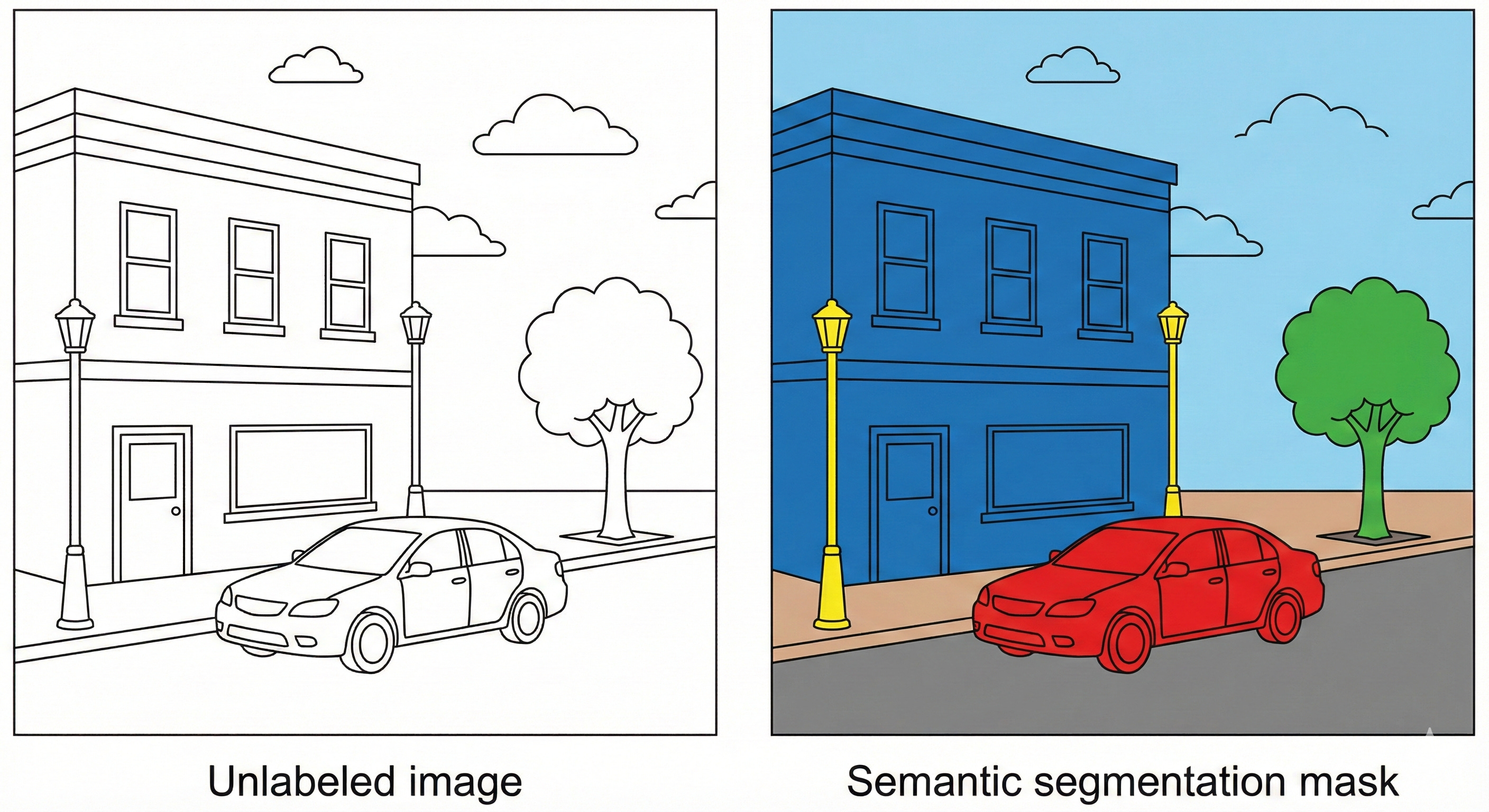
Before architectures like U-Net, deep networks tended to be good at the first task and clumsy at the second. They could tell you that the image contained a bus, but they were sloppy at outlining it. The result looked like a toddler using a thick paintbrush. Red splashed in roughly the right region, but the borders were fuzzy and imprecise.
U-Net changed that balance. It behaves more like an artist with a fine liner. The contracting path compresses the image and learns what is in the scene. The expansive path then brings the resolution back up and uses skip connections to recover fine detail, so the network can place boundaries with pixel level accuracy. The same machinery that decides “this region is bus” also learns exactly where the bus stops and the sky begins.
This blog is intended as a practical, end to end guide to U-Net. We will unpack the architecture block by block, look at the intuition behind the key equations, and examine the geometric picture of how information flows through the network. By the end, you will see why this specific layout of convolutions, pooling, upsampling, and skip connections has become the default choice for dense prediction problems in fields ranging from medicine to generative image models.
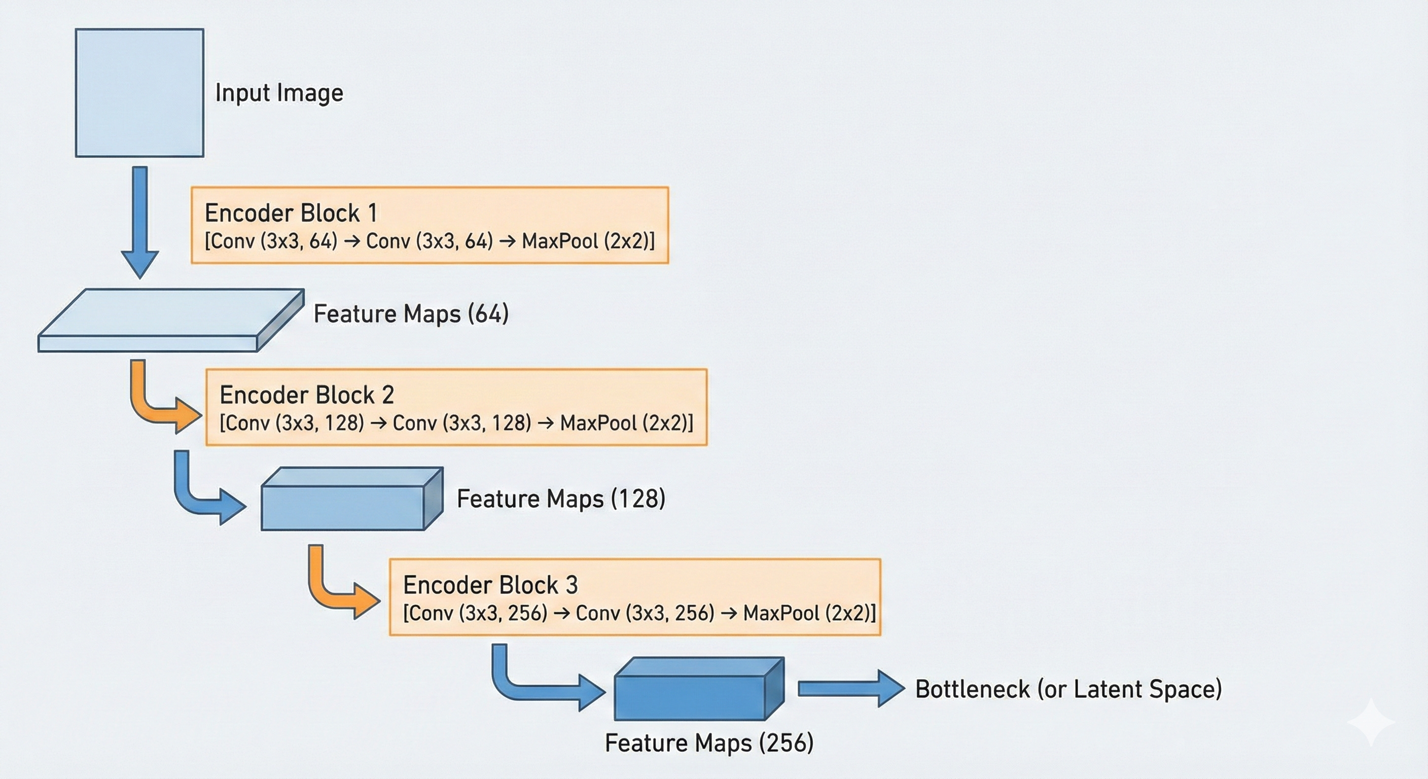
The Encoder: The Contracting Path
The first half of the U-Net, often called the encoder or contracting path, is in charge of the “what.” Its job is to ignore the irrelevant surface details of the image, such as the exact pavement texture or subtle lighting variations on a wall, and compress the input into a compact representation that captures meaning. In practical terms, it turns a high-resolution grid of pixels into a lower-resolution grid of abstract features.
Structurally, this encoder looks a lot like a standard convolutional network such as VGG-16. It is built from repeated blocks that combine two key operations: convolution and max pooling.
Convolution: the flashlight and the stencil
The basic building block of U-Net is the convolution. To make sense of it, it helps to stop thinking of an image as a picture and instead treat it as a table of numbers. A grayscale image is a grid of intensity values, where 0 might represent black and 255 white. A color image is three such grids stacked together: one for red, one for green, one for blue.
A convolution uses a small learnable matrix called a kernel or filter. In U-Net, this kernel is usually 3×3.
Visual intuition: the flashlight scanner
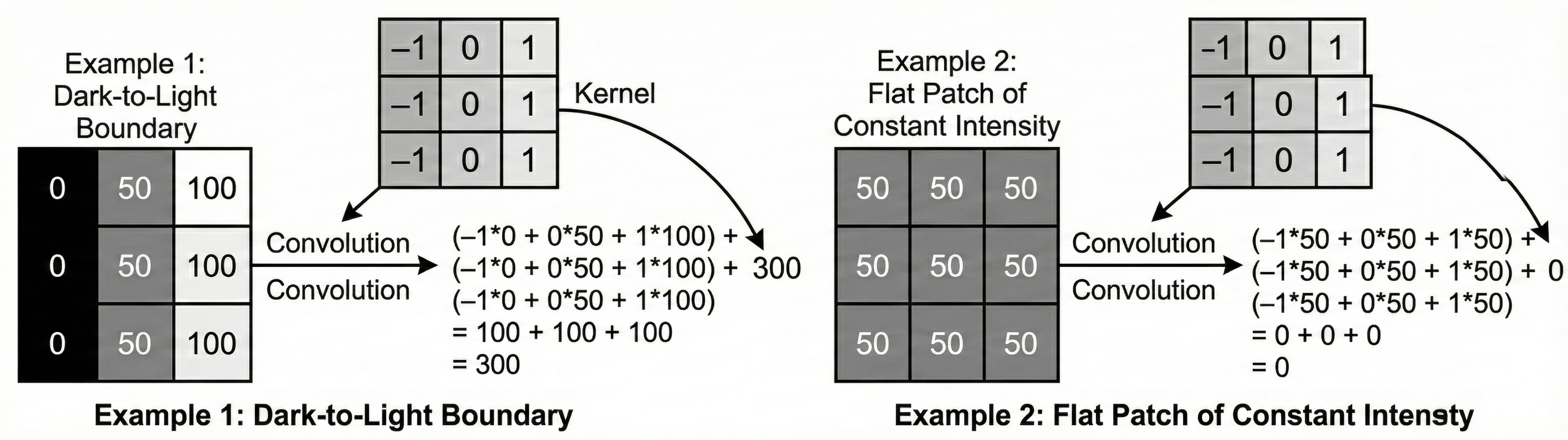
Imagine the input image painted as numbers on a large wall. The kernel is a small square flashlight that only illuminates a 3×3 patch at a time.
The flashlight starts at the top left corner and slides across the wall, one pixel at a time, until it reaches the bottom right. At each position it does something very specific: it lines up its own 3×3 numbers with the numbers on the wall, multiplies them pairwise, then adds all those products together. That single sum becomes one pixel in the output feature map.
Mathematical intuition: dot product as similarity
Under the hood, each step of this operation is a dot product between the kernel and the local patch of the image.
The intuition behind this formula is Pattern Matching. Imagine a kernel designed to detect a vertical edge. It might look like this:
Now imagine we use a very simple kernel that is designed to detect a vertical edge: negative values on the left, positive values on the right. When this kernel passes over a region of the image where the left side is dark and the right side is bright, something interesting happens.
The negative weights line up with the low pixel values on the dark side, and the positive weights line up with the high values on the bright side. When you multiply and sum: (−1×Low)+(1×High)≈Large positive value.
So the output at that location becomes a strong positive number.
If the same kernel slides over a flat region of uniform color, the story changes. The dark and bright sides are roughly the same, so the contributions from the negative and positive weights cancel out, and the result is close to zero. In other words, the kernel is “excited” only when it sees something that looks like the pattern it encodes.
This is the key idea: a convolution is not just some mechanical multiplication. It is a test. Each kernel is effectively asking every small patch of the image, “Do you look like me?” If the patch matches the pattern, the neuron produces a high response. If not, it stays quiet.
In a U-Net, these kernels are not hand-designed; they are learned from data. In the first layer, the model might learn 64 different kernels. That means the image is scanned 64 times, each pass with a different “flashlight,” each one tuned to a different pattern: vertical lines, horizontal lines, corners, small blobs of color, and so on. The result is a stack of 64 feature maps that all share the same spatial layout as the original image but no longer store raw color values. Instead, each map records where a particular learned feature is present.
The Activation: ReLU (The Gatekeeper)
After every convolution, the U-Net applies a non-linear activation function, specifically the Rectified Linear Unit (ReLU).
This formula is deceptively simple: it replaces all negative values with zero.
Why do we need ReLU at all? Without any nonlinearity, a neural network is just a chain of linear operations. If you stack one linear layer on top of another, the result is still a single linear transformation. In that world, you could replace a massive, billion parameter model with one big matrix multiplication and you would not gain any extra expressive power.
The problem is that the world is not linear. The relationship between pixel values and a label like “cancerous tumor” is full of thresholds, interactions, and complicated curves. ReLU introduces the first real bend into that mapping. It cuts off all negative responses and keeps the positive ones, which makes the overall function piecewise linear instead of a single straight line.
This has two important side effects. First, ReLU acts like a gate. Only features that produce a positive match in a neuron are allowed to move forward, everything with a negative correlation is set to zero. Second, that behavior creates sparse activations. Large parts of the network stay quiet for a given input, and only the neurons that found something meaningful fire. In the “coloring book” analogy, ReLU is what lets the model draw crisp boundaries. It supports decisions like “this is an edge” or “this is not” instead of blending everything into a soft average.
Max Pooling: The Art of Summarization
As the network moves deeper into the encoder, it needs to widen its field of view. A 3×3 kernel only sees a tiny patch of the image. That is fine for simple patterns like short edges, but to recognize something like a car the model needs to relate wheels, windows, and bumper at the same time.
Instead of making the kernels much larger, which would quickly explode the number of parameters, we make the feature maps smaller.
This is where max pooling comes in.
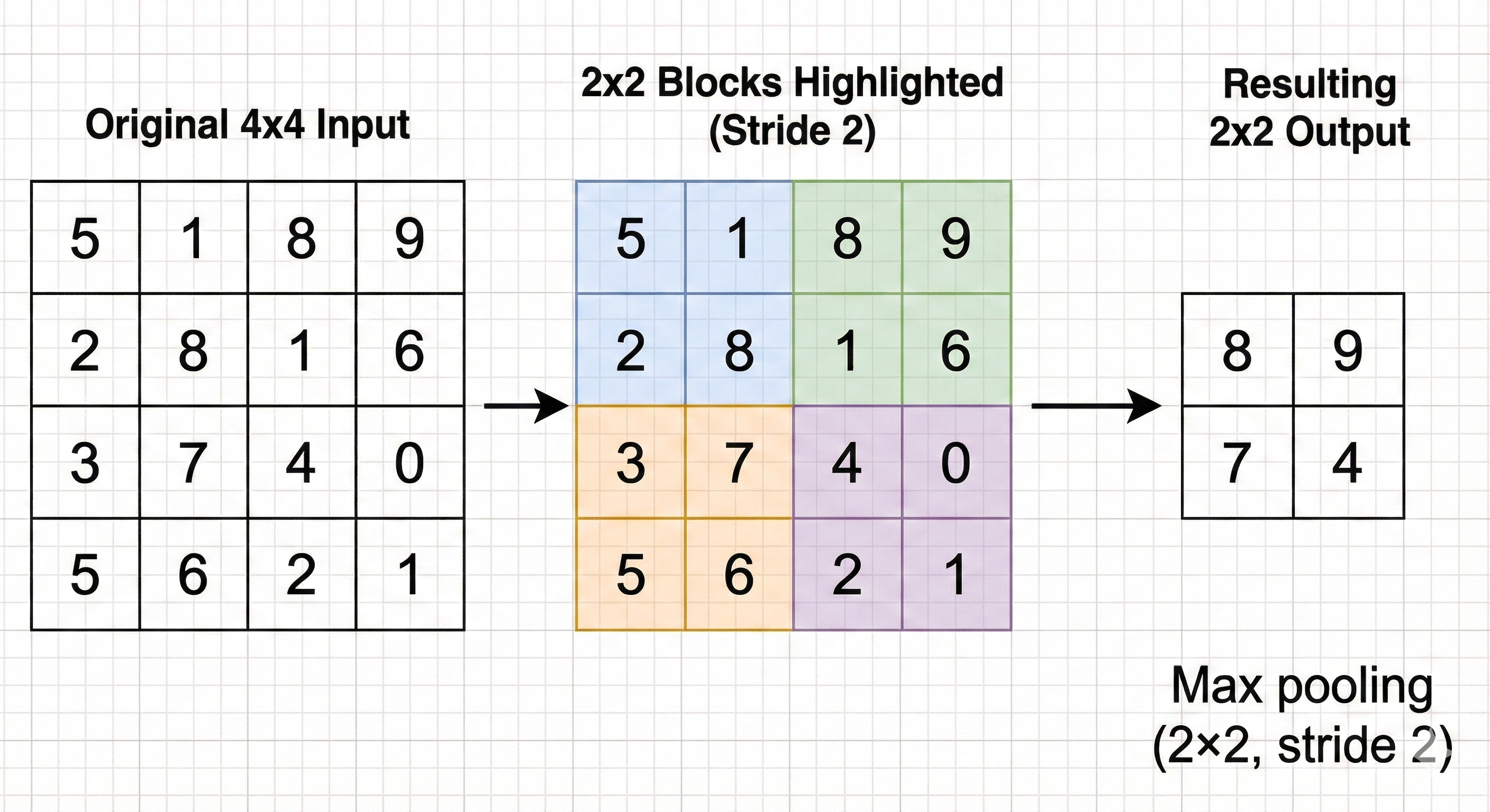
In U-Net, a 2×2 max pooling operation with stride 2 is used. The feature map is divided into non-overlapping 2×2 blocks, and in each block the operation keeps only the single largest value.
Visual concept: the pixelated mosaic
Imagine starting with a sharp, high resolution image. You lay a grid on top of it that groups pixels into 2×2 squares. In every square you identify the “loudest” pixel, the one with the strongest activation, and throw away the other three.
The resulting image is half the height and half the width of the original, but it still preserves where the strongest responses were.
Why max pooling helps, and what it breaks
Translation invariance.
This is the main benefit. If a small feature such as the tip of a cat’s ear moves by one pixel, it will probably still land inside the same 2×2 pooling window. The maximum value in that window will not change much, so the representation is stable under small shifts and distortions.
Receptive field expansion.
By shrinking the feature maps, the next 3×3 convolution effectively covers a larger region of the original input. After several rounds of pooling, a single activation deep in the encoder corresponds to a large patch of the original image. This is what lets the network reason about whole objects rather than just tiny fragments.
Losing the “where.”
The tradeoff is that max pooling throws away spatial detail. Keeping only one value out of four means losing 75 percent of the local information. You still know that “some edge exists in this 2×2 block,” but you no longer know its exact location inside the block.
That loss of precise position is the core problem that the second half of the U-Net, the decoder or expansive path, is designed to fix.
The Bottleneck: The Latent Representation
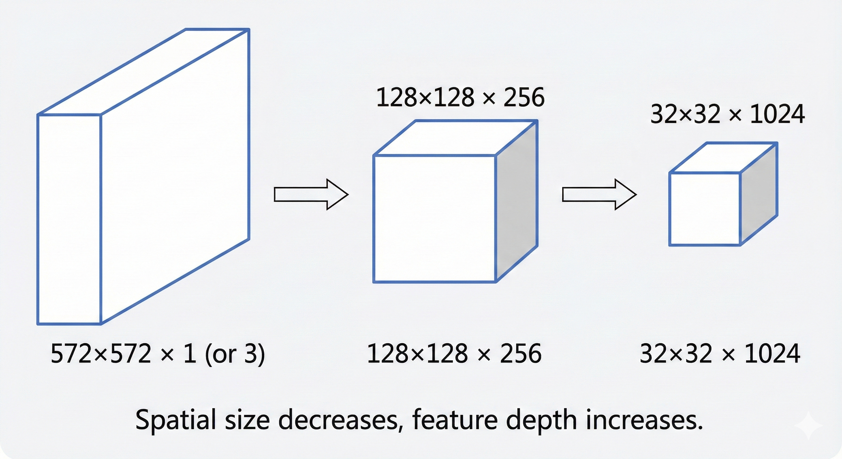
At the bottom of the U-shape sits the bottleneck. By this point, the image has gone through several rounds of max pooling. In the original U-Net specification, an input of 572×572 pixels is reduced to a compact grid of about 32×32.
The resolution is now very low, but the depth of the features is extremely high. The bottleneck often carries 1024 separate channels. That means each location in this 32×32 grid is represented by a vector of 1024 numbers. These values no longer encode simple properties such as raw color or brightness. They correspond to abstract concepts such as “fur-like texture,” “metallic surface,” “organic contour,” or “open sky.”
You can think of this bottleneck as a compressed summary. It plays a role similar to a zip file or a short executive brief. Almost all of the information about what is in the image is still present (for example, “there is a cat in the lower left and a tree in the upper right”), but the fine-grained layout of individual pixels has been stripped away. In the language of modern generative models, this region of the network is a latent space, a mathematical place where the idea of the image lives, separate from its exact pixel-level appearance.
For the U-Net, this is the turning point. Up to the bottleneck, the encoder has focused on answering “What is in this image?” From this point on, the decoder has to take that compressed understanding and map it back to “Where is everything, exactly?”
The Decoder: The Expansive Path
The second half of the U-Net, often called the decoder or expansive path, is essentially a mirror of the encoder. Its job is to take the compact, abstract representation from the bottleneck and gradually stretch it back out to the original resolution of the input image. Along the way, it has to restore the spatial detail that was stripped away by max pooling.
To do this, it leans on two key steps at each level of the “U”:
Upsampling, to increase the spatial size of the feature maps.
Concatenation via skip connections, to bring back fine-grained details from the corresponding encoder layer.

Upsampling: The Inverse of Pooling
How do we actually make a small feature map bigger again?
In U-Net style architectures there are two common strategies, and the choice between them has a direct impact on the quality of the final segmentation.
Method A: Transposed Convolution (learnable upsampling)
In the original U-Net paper, the decoder uses transposed convolutions (often called “deconvolutions,” although that is technically a misnomer).
Intuition
A standard convolution takes a local patch of pixels and compresses it into a single value. This is a many-to-one operation.
A transposed convolution does the opposite. It starts from one value and spreads it out into a small patch. This is a one-to-many operation.
How it works
The network learns a kernel that behaves like a stamp. For every pixel in the smaller feature map, that kernel is “stamped” onto the larger output map.
If the input pixel has a high value, the stamp is pressed hard and the resulting pattern has high intensity.
If the pixel has a low value, the stamp is faint.
By sliding this learnable stamp over the low-resolution feature map with a certain stride, the network constructs a higher resolution feature map.
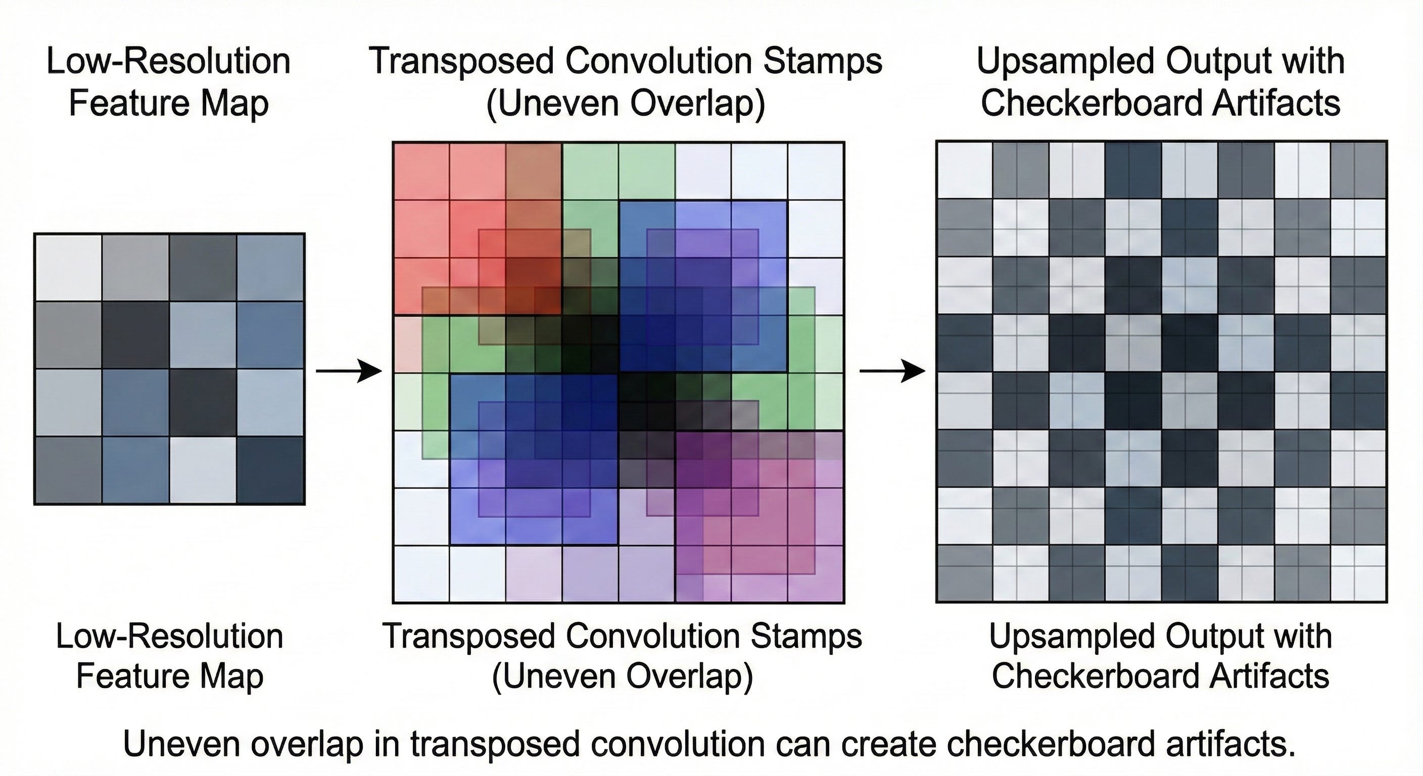
The artifact problem
Transposed convolutions are infamous for introducing checkerboard artifacts.
If the stride does not divide the kernel size evenly, some locations in the output receive overlapping contributions from multiple stamps while others receive fewer. A few pixels get hit twice, others once. The result is a subtle grid pattern that shows up in the final prediction. It looks unnatural and can distort boundaries in segmentation maps.
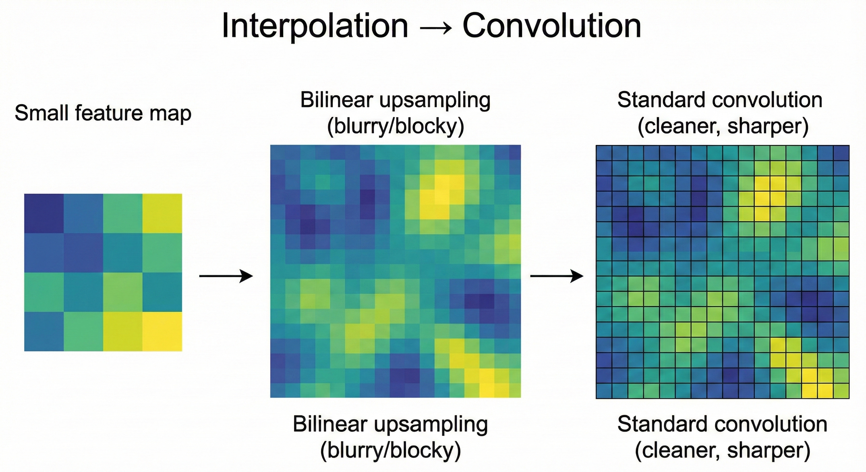
Method B: Bilinear Upsampling + Convolution (modern default)
To avoid these artifacts, many modern U-Net implementations, including those inside diffusion models, use a two-stage approach:
Interpolation (nearest-neighbor or bilinear)
The feature map is first resized to the target resolution using a standard interpolation method. This step is purely mathematical. No learning takes place here. The operation simply stretches the grid to the new size.Standard convolution
Right after resizing, a regular convolution layer is applied. This layer is learnable and is responsible for refining the upsampled features and smoothing out any blocky artifacts created by interpolation.
Why this tends to work better
By separating “make it bigger” from “learn useful features,” the network becomes easier to control.
The interpolation step guarantees a clean, uniform resizing.
The following convolution can then focus exclusively on shaping and sharpening the features.
In practice this combination produces smoother, more stable, and artifact-free segmentation maps.
The Skip Connections: The Teleportation Bridges
If U-Net only had an encoder and a decoder, it would not work nearly as well. The bottleneck is a lossy compression. When you stretch a 32×32 representation back out to 572×572, the result will naturally be soft and blurry. The network might know that “there is a car in this region,” but it no longer remembers the exact pixel where the bumper ends and the road begins.
This is exactly why skip connections are the key idea in U-Net.
Skip connections: bringing back the missing detail
Visual concept: the transparency overlay
Imagine you are trying to restore a damaged painting. The restored version has the rough shapes in place but is missing the fine brushstrokes. Somewhere in the archive, however, you have a transparent sheet with the original fine-line work.
A skip connection plays the role of that overlay. The “damaged painting” is the coarse feature map coming up from the bottleneck. The “overlay” is the high resolution feature map stored in the encoder before pooling.
At each stage of the decoder, U-Net finds the encoder layer that had the same spatial resolution. It then takes that encoder feature map and concatenates it with the current upsampled decoder feature map.
Concatenation vs. addition: how U-Net differs from ResNet
It is important to distinguish U-Net’s skip connections from those in ResNet:
ResNet uses addition:
\(Output=Input+F(Input)\)This keeps the signal magnitude stable and helps gradients flow through very deep stacks of layers.
U-Net uses concatenation:
The feature maps are stacked along the channel dimension. If the decoder tensor has 256 channels and the encoder skip contributes another 256, the combined tensor has 512 channels.
Concatenation has a specific benefit in the segmentation setting. It lets the network put context and local detail side by side. The decoder channels say “this region belongs to a car,” while the encoder channels provide sharp local cues like “there is a strong edge exactly here.” The following convolutional layers can look at both sources at once and decide: “This is a car boundary, and this pixel lies exactly on the edge, so I should draw the border right here.”
Without these skip connections, the model behaves like a blurry autoencoder. With them, it becomes a tool that can lock boundaries down to individual pixels.
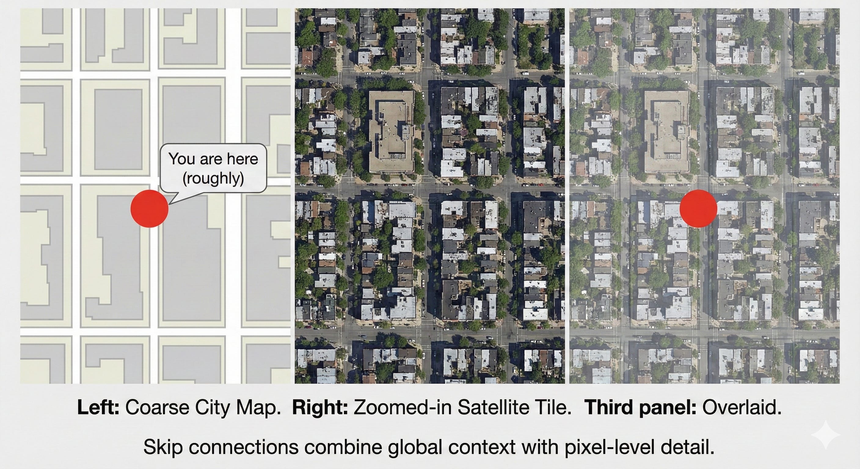
Visual concept: the GPS analogy
The bottleneck is like a GPS that tells you “you are somewhere in New York City.” It has a lot of context but very little precision.
An early encoder feature map is like a detailed satellite view that shows the curb, the crosswalk lines, and the exact shape of the street. It has high precision but no global story.
A skip connection is what happens when you overlay the satellite image on top of the GPS map. You know both where you are in the city and exactly where to stand on the sidewalk.
Training the U-Net: Loss and Optimization
An architecture is only as good as the signal used to train it. For U-Net, choosing the right Loss Function is critical, especially given the domain of medical imaging where data is often sparse and imbalanced.
The Imbalance Problem
In many medical images, the thing we care about is extremely small. In a brain scan, a tumor might cover only one percent of the pixels. The remaining ninety-nine percent is healthy tissue or background.
If we train a model and judge it using plain pixel accuracy, it can reach 99% accuracy by predicting “no tumor” everywhere. From a spreadsheet point of view this looks excellent. From a clinical point of view it is disastrous.
This is the core imbalance problem in segmentation. The positive class is tiny. A naive metric will reward models that ignore it.
The Dice Coefficient (Sorensen–Dice Index)
To address this, U-Net models are often trained with Dice loss, which is based on the Dice coefficient. Instead of counting how many pixels were classified correctly, it measures how much the predicted mask overlaps the ground truth.
Intuitively, Dice asks “How big is the intersection compared to the total area covered by either mask?” A perfect overlap gives a score of 1. No overlap at all gives 0.
For two sets of pixels, A (ground truth) and B (prediction), the Dice coefficient is
Here, P is the set of pixels predicted as positive by the network, and T is the set of ground truth (target) positive pixels.
You can think of the Dice coefficient as “intersection over total.”
The numerator, 2∣P∩T∣, counts how many pixels the prediction and the ground truth agree on. We multiply by 2 because those overlapping pixels appear once in ∣P∣ and once in ∣T∣ in the denominator.
The denominator, ∣P∣+∣T∣, is simply the total number of pixels marked as positive in either mask.
This is why Dice is so useful for highly imbalanced problems. Predicting the background correctly does not boost the score. The Dice value moves only when the model does a better job of capturing the tumor itself.
If the tumor occupies 10 pixels and the network correctly finds 5 of them, the Dice score reflects that partial overlap directly, without being diluted by the millions of background pixels. As a result, gradient descent is pushed to focus on the structure of interest instead of being rewarded for saying “background” everywhere.
Data Augmentation: The “Jelly” Deformations
One of the more surprising observations in the original U-Net paper was how well it could perform with very little labeled data. In some biomedical benchmarks, the model was trained on as few as 30 images. The key to making this work was aggressive data augmentation.
In medical imaging, most structures are soft and deformable. A cell is still a cell if it is slightly stretched, compressed, or rotated. U-Net takes advantage of this by applying elastic deformations to the training images.
Visual concept: The jelly sheet
Imagine printing a microscopic image onto a sheet of jelly. You then poke, pull, twist, and gently stretch the jelly in different directions. The overall content is the same, but the exact shape and position of each cell changes in subtle ways.
From a single labeled image, this process can generate thousands of realistic variations. The model is forced to learn properties that survive these distortions, such as the texture and boundary characteristics of a cell wall, rather than memorizing a single fixed outline. This emphasis on shape- and deformation-invariant features is a major reason U-Net became the default choice for medical imaging tasks, where labeled data is scarce and biological structures are rarely rigid.
The Modern Era: U-Net in Generative AI (Stable Diffusion)
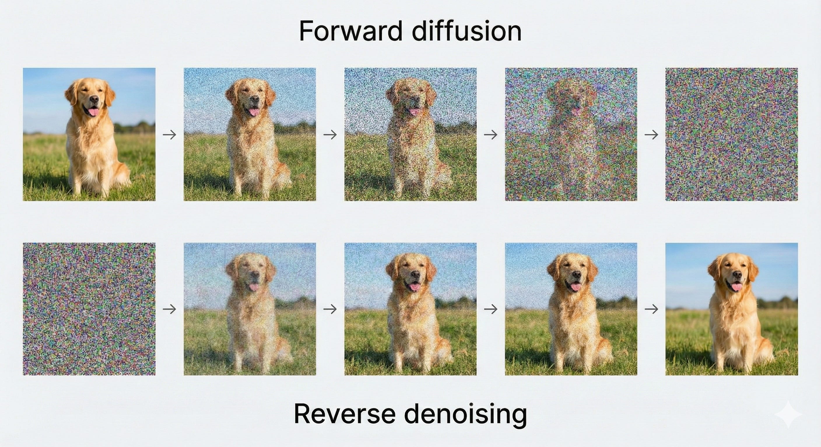
While U-Net originally rose to prominence in medical imaging, its most widely known role today is in diffusion models such as Stable Diffusion. In this context, the U-Net is repurposed. Instead of outlining tumors, it learns to predict noise.
The diffusion process: from image to noise and back
Diffusion models follow a simple idea, applied step by step.
Forward process
Start with a clean image and gradually add Gaussian noise over many steps, until the image becomes essentially pure static.Reverse process
Train a neural network to look at a noisy image and estimate the noise that was added at each step so that it can be subtracted, slowly revealing a clean image again.
Why is U-Net a natural choice here?
At each reverse step, the task looks like this:
Input: a noisy image of size 512 × 512
Output: a predicted noise map of size 512 × 512
The input and output share the same spatial layout. The network must understand global structure (“there is a face here, a horizon there”) and at the same time make pixel-level judgments (“this exact pixel is noise, not part of an eye”). That combination of global understanding and precise localization is exactly what U-Net is designed to handle.
Adapting U-Net for image generation
To work inside Stable Diffusion–style systems, the basic U-Net is extended with two important components: a notion of time and a way to incorporate text prompts.
1. Time embeddings: giving the network a clock
The U-Net needs to know how noisy the current image is. An early reverse step, where the image is almost pure static, is a very different situation from a late step, where most of the structure has already been recovered.
When the noise level is very high (for example, time step t ≈1000), the model should focus on broad, low-frequency structure.
When the noise level is low (for example, time step t ≈ 10), it should refine fine textures and small details.
To give the model this sense of “where we are in the process,” a time embedding is created from the current timestep. This is often done using sinusoidal functions, in a way similar to positional encodings in Transformers. The resulting vector is then projected to the right dimension and added into the intermediate feature maps inside the U-Net’s residual blocks.
In effect, the time embedding tells the network how aggressively to denoise and what kind of features to pay attention to at that stage.
2. Cross-attention: injecting the text prompt
The next question is how the network knows to produce a “cat on a beach at sunset” rather than a “car in the rain.” This is where cross-attention comes in.
First, the text prompt is passed through a text encoder such as CLIP or a Transformer-based model. This turns the sentence into a set of vectors that encode its meaning.
Inside the U-Net, cross-attention layers are added, often around the bottleneck and in the deeper decoder blocks. These layers let the visual features “look up” information from the text features.
As the U-Net processes the noisy image, the cross-attention mechanism allows each spatial location to query the text representation. Conceptually, a region in the feature map can ask the prompt, “Does what I am seeing here match the word ‘cat’ or the word ‘sky’?” The text then guides the reconstruction, nudging the network to clean up the noise into shapes, colors, and textures that match the description.
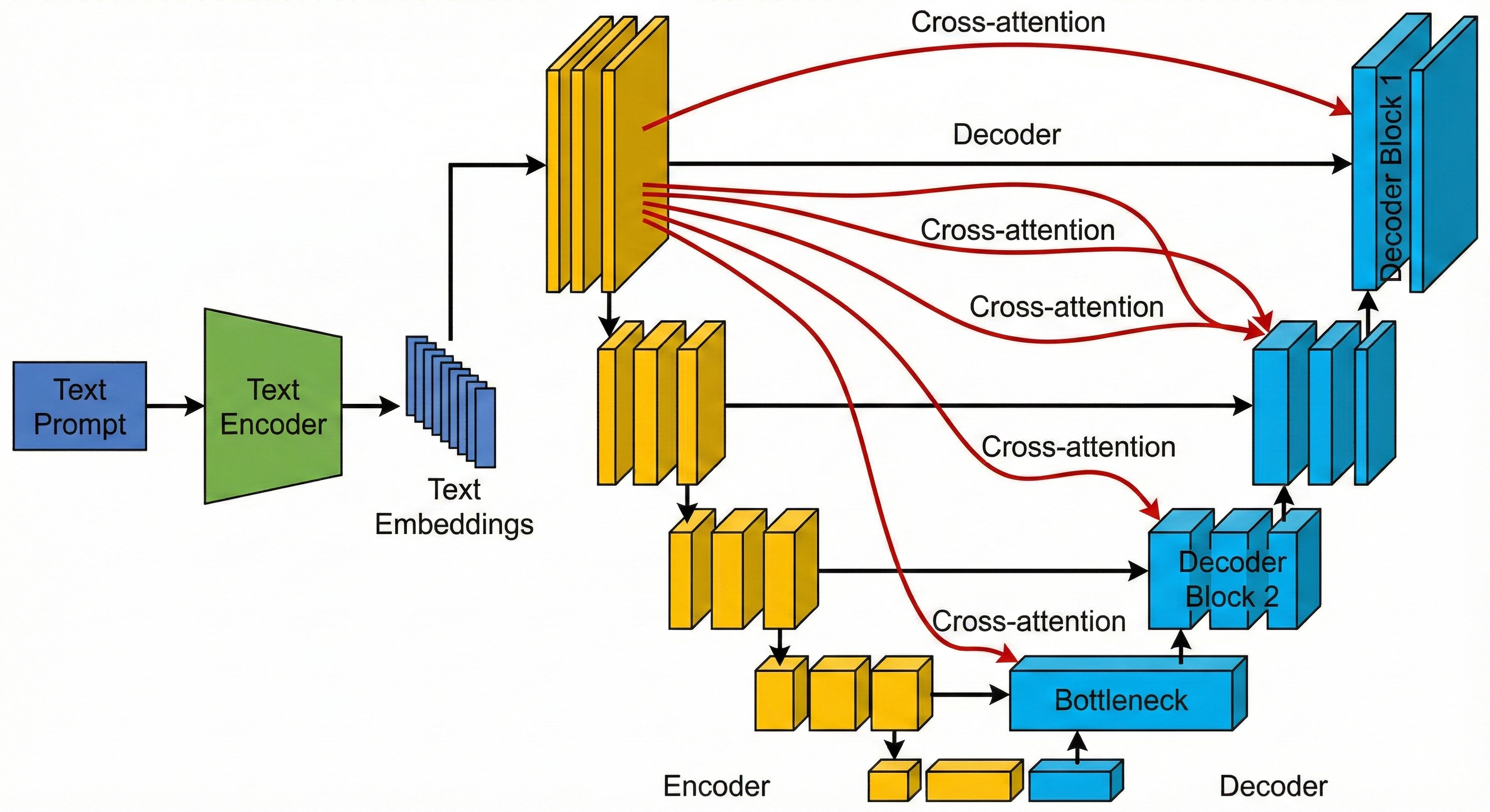
In this way, the U-Net that once traced the outline of tumors is now used to sculpt images from randomness. Time embeddings tell it how far along the denoising schedule it is, and cross-attention tells it what the image should depict. Together, they turn the U-shaped architecture into the workhorse of modern text-to-image generation.
Conclusion: The Unreasonable Effectiveness of the U-Net
The U-Net is a good example of how far you can go with a simple idea used well. It builds its power on symmetry: one path that contracts to capture context, and a matching path that expands to recover detail. In doing so, it reflects a basic requirement of visual understanding: we need to see both the forest and the trees.
Its core principles of compressing information into a bottleneck, retrieving detail through skip connections, and processing features at multiple scales have held up far beyond the original goal of biomedical segmentation. The same pattern now appears in systems that help cars follow lane markings, satellites track changes in forests, and generative models turn text prompts into images, whether that prompt describes a tumor, a cityscape, or an astronaut on a horse.